

On this page
A salt marsh protects the dike behind it only as long as it keeps up with the sea. Whether it does comes down to a sediment budget measured in centimetres: mud settling on the flats in front of the marsh, and the marsh edge crumbling where waves attack it.
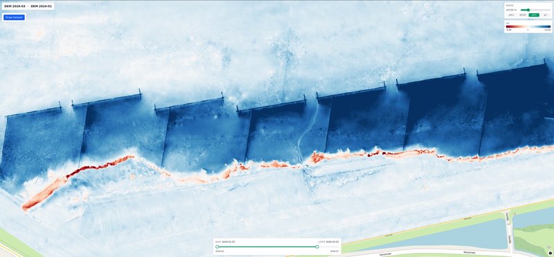
At Wierum, on the Frisian coast of the Wadden Sea, we measured those changes across the whole site for CODAP, the Coastal Data Portal we built with Rijkswaterstaat and Lumax AI. Between January 2024 and March 2026, half of the site rose by 11 cm or more, and the fields between the brushwood groynes by up to about half a metre. Along the marsh edge, a narrow band dropped by up to about 50 cm.
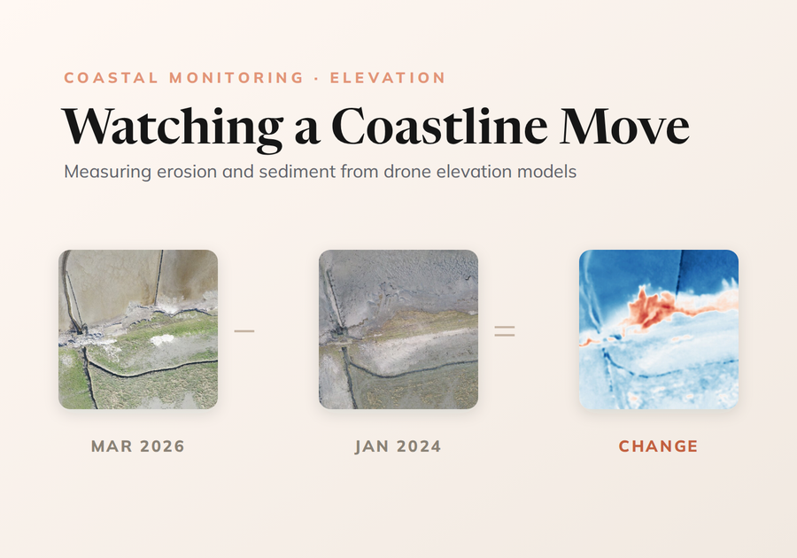
This post is about how those numbers are made: from drone photos to elevation models, from two elevation models to a map of change, and from a map of change to a reading of the coast.
From drone photos to an elevation model
Each drone survey produces many overlapping photos. Photogrammetry matches the same points across photos taken from different positions and reconstructs the surface in 3D. The same processing that gives the orthophoto, the distortion-free aerial photo used for land-cover mapping, also gives a digital elevation model (DEM): a raster that stores the height of every point on the site.
For change detection, the DEM is what matters. One DEM is a snapshot. Two DEMs of the same place, on different dates, are a measurement.
The DEM of difference
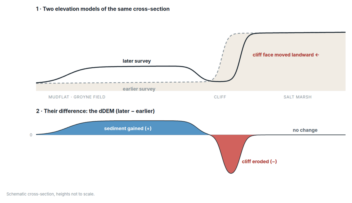
Subtracting the earlier DEM from the later one, pixel by pixel, gives a DEM of difference, or dDEM:
- positive where the ground rose: sediment was deposited;
- negative where it dropped: erosion;
- around zero where nothing changed.
The operation is simple. Everything around it needs care. Both DEMs have to line up exactly, so that every pixel compares the same spot on the ground. And a coast is only understood by comparing many moments, so we compute a dDEM for every pair of surveys: six surveys give fifteen pairs, and the portal can compare any two dates.
Signal and noise
A photogrammetric DEM is not perfect. Every surface carries a little noise, and subtracting two of them adds their noise together. We measured it on one pair of surveys:
| What we measured | Size |
|---|---|
| Typical spread of the change across the site | ±4.5 cm |
| Typical difference between neighbouring pixels | 5 mm |
| Sparse spikes (1st to 99th percentile of pixel-to-pixel jumps) | ±3 to 4 cm |
So the dDEM is a smooth field of centimetre-scale change, with sparse spikes of the same size scattered on top. The spikes are the problem: to see centimetres, the colour scale has to be stretched hard, and the stretch turns them into a salt-and-pepper texture that hides the pattern.
The way out is that real change is spatially coherent, and noise is not. Erosion and deposition affect patches of ground, many pixels at once. A spike affects one pixel. That difference is what the filter uses:
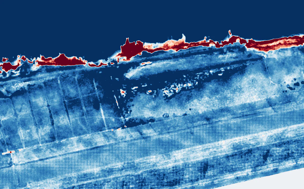
- Median despike. Each pixel is compared with the median of its 5 × 5 neighbourhood. If it differs by more than 3 cm, it is replaced by that median. A single-pixel spike is removed; a patch of real change, which moves its whole neighbourhood, is left alone.
- Light smoothing. A Gaussian blur with σ = 1 pixel (about 40 cm) reduces the remaining 5 mm wobble.
Pixels with no data stay empty in the result, so the filter never adds values where the survey has none. The settings were chosen by comparing a few variants side by side on one pair before processing all fifteen.
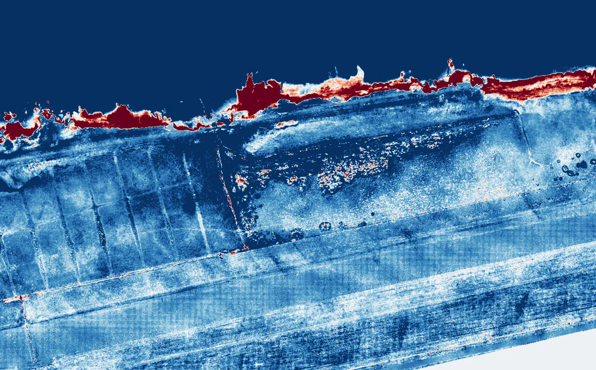
 Raw dDEM
Filtered
Raw dDEM
Filtered
The main thing lost is a genuine change confined to a single 40 cm pixel. That sits at the level of the noise itself, so it could not have been trusted anyway.
Reading the coast with transects
A map of change shows where to look. A transect shows how much. The portal serves the change maps as image tiles that carry the height of every pixel, precise to about 4 mm, so the colour range can be changed instantly and transects can be read straight from the map. In the Erosion tab, anyone can draw a line across the map and get a profile of the height change along it.
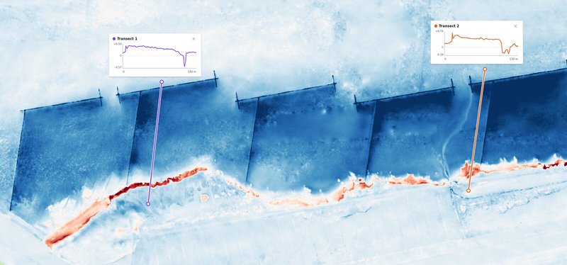
At Wierum, the profiles tell a consistent story: the ground rises across the groyne fields, then drops sharply where the line crosses the marsh edge. Where sediment builds up and where the cliff retreats is exactly what a coastal manager needs to know. A structure was built at Wierum to protect the marsh cliff from erosion, and the change map and transects show within minutes where sediment is building up and where the cliff is still retreating.
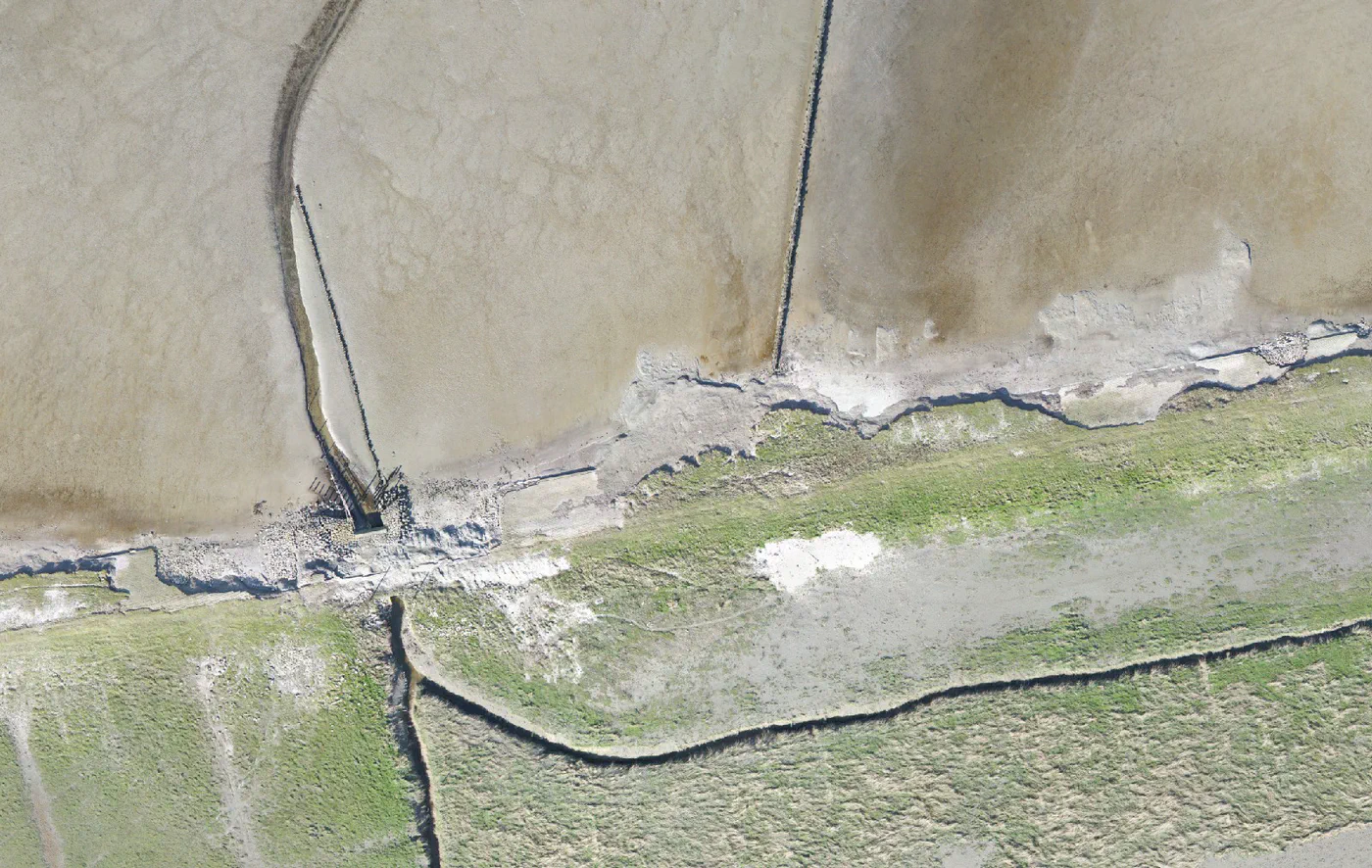
The photos show the same thing. Drag across the same 120 m of cliff, two winters apart:
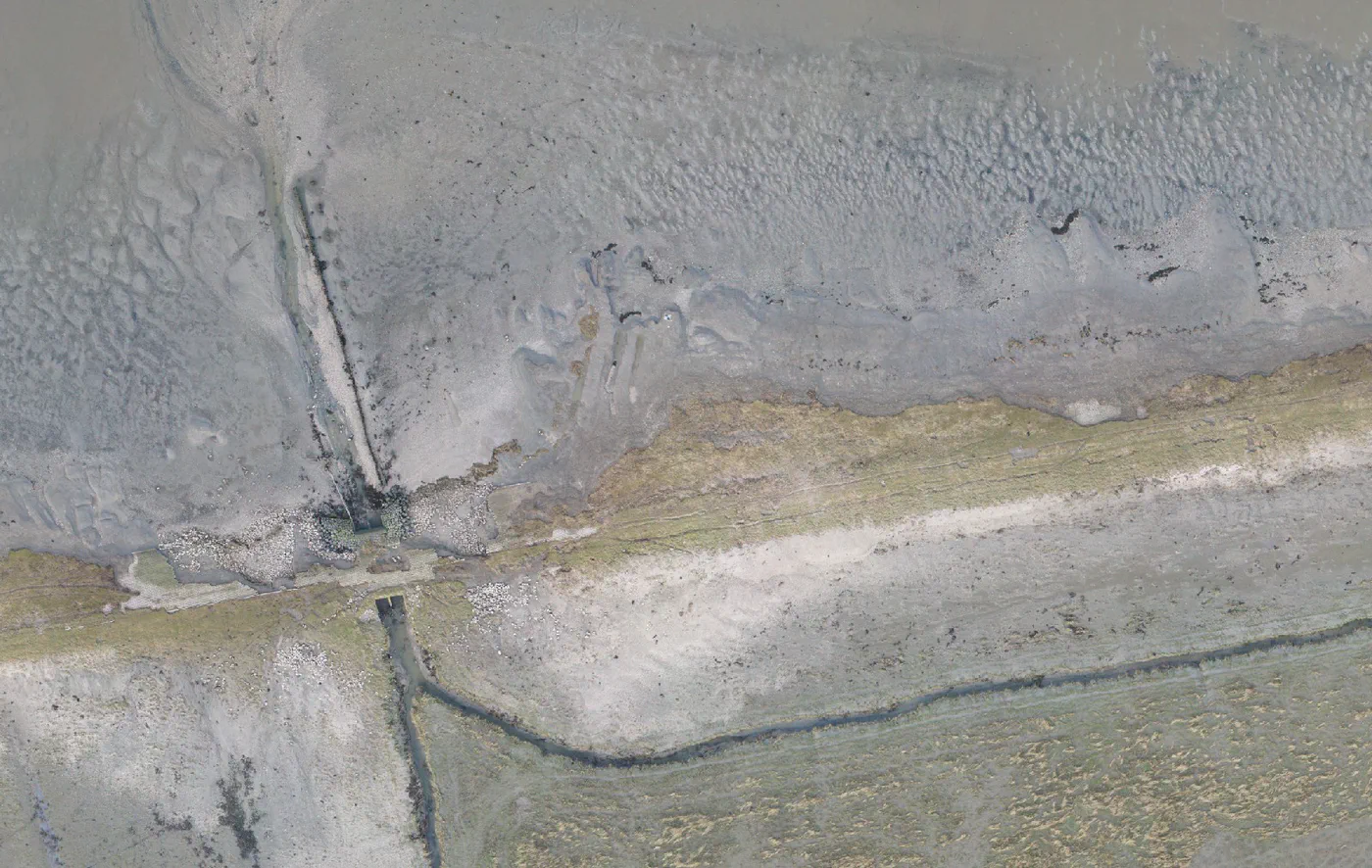
 Jan 2024
Mar 2026
Jan 2024
Mar 2026
The same spot, six times
Two surveys show a difference. Six show a trend. Here is the same 100 m by 70 m of cliff and groyne field in every survey, with the change since the first survey underneath, and the median change over time for two parts of it: the groyne field, and the patch of cliff that had dropped by more than 15 cm by March 2026.
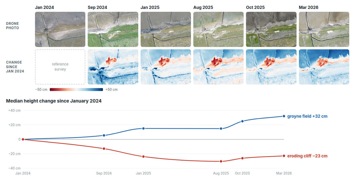
The groyne field rose in steps, to +32 cm by March 2026. The cliff patch dropped fast, to −30 cm by August 2025, then partly filled back in, to −23 cm by March 2026. A single pair of surveys shows only the net result; the series shows how it happened, and when.
What’s next
Change maps answer “where” and “how much”. The next step is combining them with the land-cover maps to answer “what”: how much of the eroding band is salt marsh and how much is bare mud, and where sediment is settling on vegetation. After that come volumes and sediment budgets per groyne field, and more sites along the Wadden Sea. Adding a survey is routine: every new flight adds a new set of pairs to compare.
Explore the live portal
The CODAP portal is public. Open the Erosion tab, pick any two surveys, and draw your own transects across the Wierum coast.
Open the portal