Welcome to our blog post where we’ll explore the development process of a benthic coral reef analyzer, created in partnership with ReefSupport. Our goal is simple: to improve the tools available for monitoring coral reefs and marine environments. Let’s dive into how we’re making this happen!
For a comprehensive understanding of this project, please click on the image below:
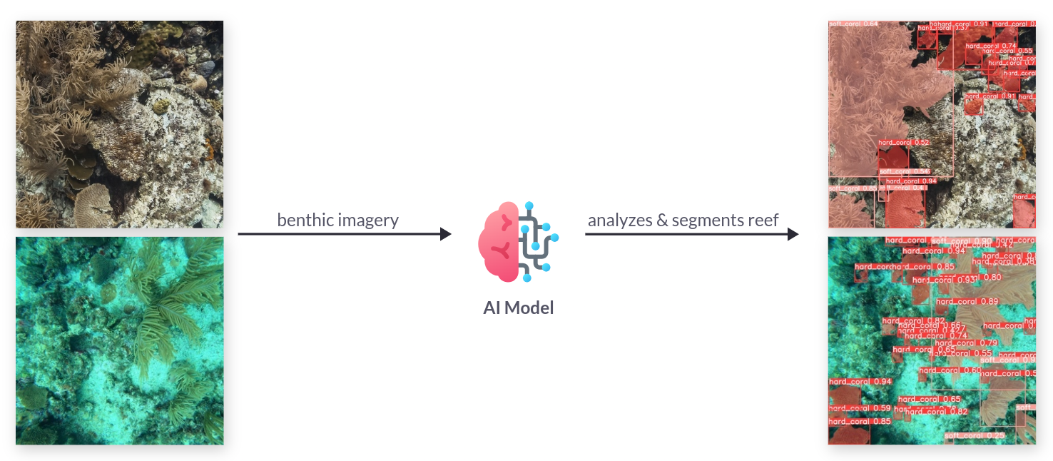
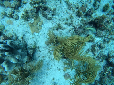
Leveraging computer vision for the segmentation of coral reefs in benthic imagery holds the potential to quantify the long-term growth or decline of coral cover within marine protected areas
Project Scope
Our collaboration aims to lead the way in developing an advanced underwater benthic imagery model. This model is designed to accurately identify and locate various functional groups within reef ecosystems. It’s flexible and can be used in different marine regions worldwide.
 Gallery / Benthic Imagery Analysis System by Reef Support
Initially, our main focus is on distinguishing between hard and soft coral species. However, our approach is iterative, meaning we can gradually include more detailed taxonomic classifications as the system evolves and becomes more sophisticated. By establishing a strong foundation with this broad framework, we set the stage for comprehensive analysis and management of reef ecosystems.
Provided Datasets
The data provided by ReefSupport is made available on a publically hosted Google Cloud bucket. Two types of datasets are available:
- Point Labels or Sparse Labels: random points in an image are classified. A typical image would contain between 50 and 100 point labels.
- Mask Labels or Dense Labels: detailed segmentations masks are
provided for hard and soft corals.
- CoralSeg
- ReefSupport meticulously annotated subsets of the aforementioned datasets, ensuring comprehensive coverage of coral reefs spanning various global regions.
Each image is associated with a dense stitched mask made of all the individual coral instances.
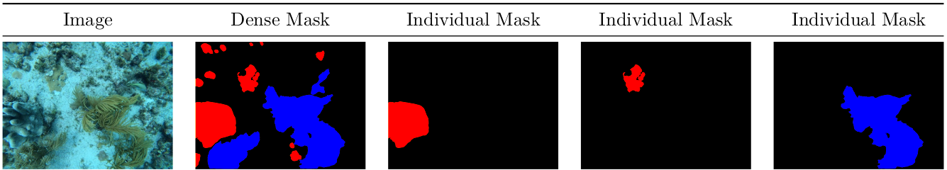 Associated labels from the ReefSupport dataset - hard and soft coral instances masks
Exploratory Data Analysis
Exploratory Data Analysis (EDA) is an approach to analyzing datasets to summarize their main characteristics, often employing visual methods. The primary goal of EDA is to uncover patterns, relationships, and anomalies in the data, which can then inform subsequent analysis or modeling tasks.
EDA typically involves the following steps:
- Data Collection: Gathering the relevant dataset(s) from various sources.
- Data Cleaning: Identifying and handling missing values, outliers, and inconsistencies in the data.
- Summary Statistics: Computing descriptive statistics such as mean, median, mode, standard deviation, etc., to understand the central tendencies and variability of the data.
- Data Visualization: Creating visual representations of the data using plots, charts, histograms, scatter plots, etc., to explore patterns, distributions, correlations, and trends within the data.
- Exploratory Modeling: Building simple models or using statistical techniques to further understand relationships within the data.
- Hypothesis Testing: Formulating and testing hypotheses about the data to validate assumptions or gain insights.
- Iterative Analysis: Iteratively exploring the data, refining analysis techniques, and generating new hypotheses as insights emerge.
EDA is a crucial initial step in any data analysis or modeling project as it helps analysts gain a deeper understanding of the dataset, identify potential challenges or biases, and inform subsequent analytical decisions. It provides a foundation for more advanced analyses, such as predictive modeling, hypothesis testing, or machine learning, by guiding feature selection, model building, and evaluation strategies.
Data quality issues
This section outlines various data quality issues identified during the Exploratory Data Analysis (EDA) process.
Empty masks
Empty stitched masks, characterized by entirely black pixels, were identified within the datasets. Subsequent removal of these empty masks resulted in improved overall performance. Notably, there were 532 empty masks identified in SEAVIEW_PAC_USA and 328 in SEAVIEW_ATL. The elimination of such empty masks contributes to a more refined dataset, enhancing the model’s efficiency and accuracy during training and evaluation.
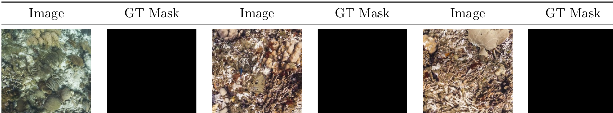 Empty Masks samples
Low quality labels
The presence of dense labels in SEAVIEW/PAC_USA has introduced challenges in the data modeling process, necessitating their exclusion from the training set. Regrettably, the labeling process for this dataset involved creating extensive masks that covered almost all corals within an image, rather than generating individual masks for each distinct entity.
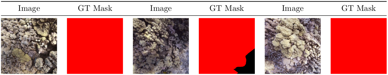 Low quality Masks samples
Mismatched sparse and dense labels
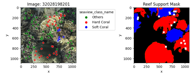
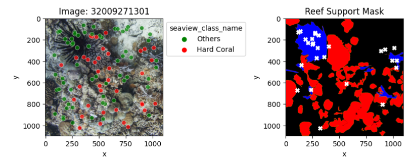
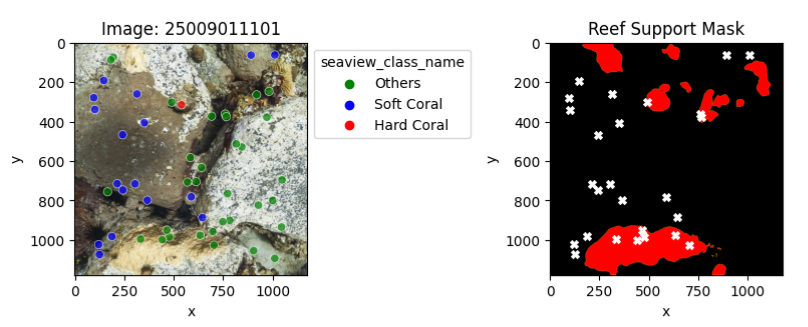
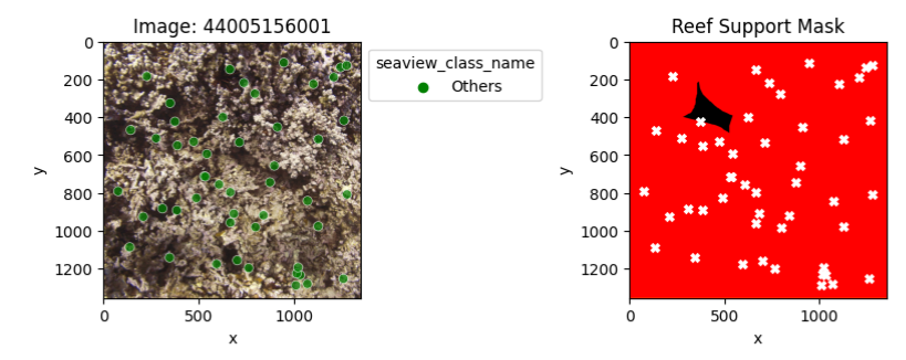
An exploratory analysis was conducted to compare sparse (point) and dense (mask) labels. In particular, we compared the dense labels provided by ReefSupport with the point labels associated with the corresponding images.
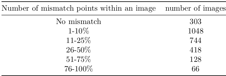
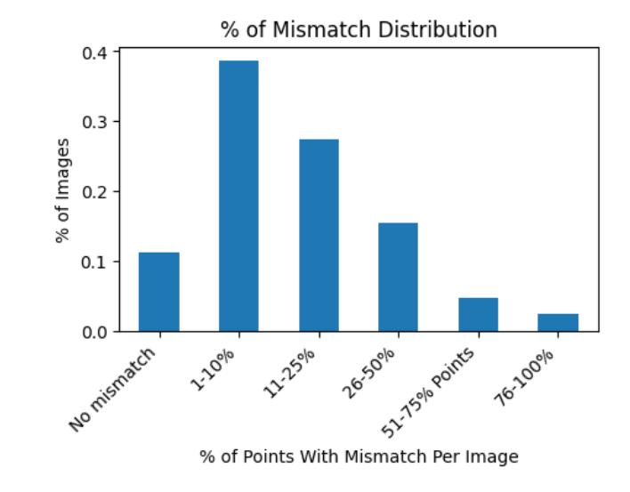
The presented samples illustrate instances where point labels contradict dense labels. Each white cross signifies a label mismatch, with the first sample showing a 17% error mismatch and the last sample demonstrating a complete 100% error mismatch.
Data leakage
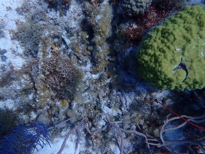
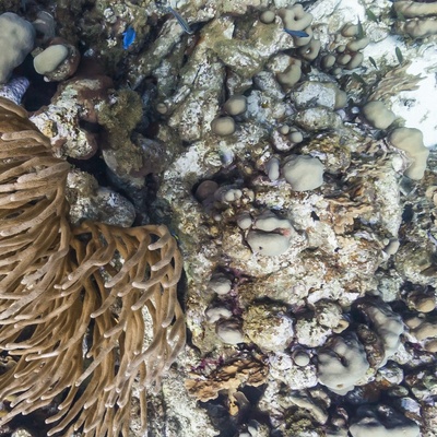
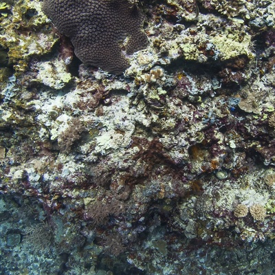
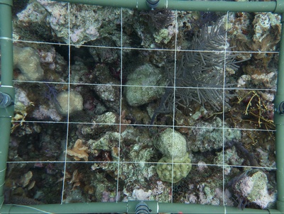
In one of the regions, certain images have been flagged for potential data leakage due to overlapping content within the same quadrats. This poses a significant challenge as these images may inadvertently find their way into multiple datasets, including training, validation, or testing sets. Such occurrences can lead to an overestimation of performance metrics during evaluations on both test and validation sets. A detailed analysis of the sequential order of image IDs highlights a consistent trend, showing that a majority of images share overlaps with their neighboring counterparts.
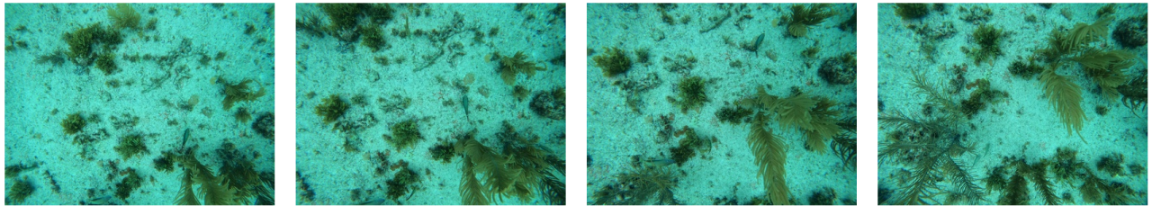 Sequence of 4 photos that share overlaps with their neigbors
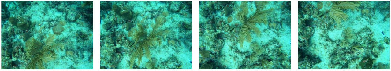 Other sequence of 4 photos that share overlaps with their neigbors
We will assess the magnitude of the data leakage by evaluating the performance of the fine-tuned model at the regional level as it only occurs in one identified region.
Class imbalance
The dataset exhibited a bias towards hard coral instances, with their prevalence being approximately five times higher compared to that of soft coral instances.
Imbalanced datasets pose challenges in machine learning, particularly when one class is substantially more dominant than others. This disparity can result in biased models that inadequately address minority classes, impacting overall performance.
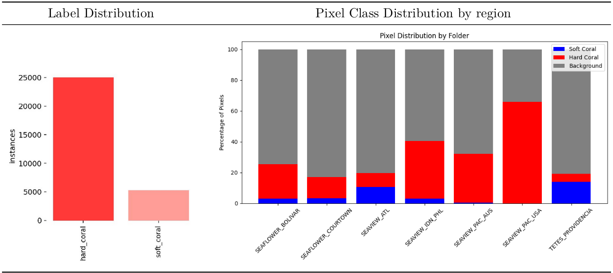 Class imbalance distributions
Data Preparation
YOLOv8 TXT format
To leverage the YOLOv8 ecosystem, it is imperative to preprocess the raw datasets provided into a format that is compatible with the model’s requirements.
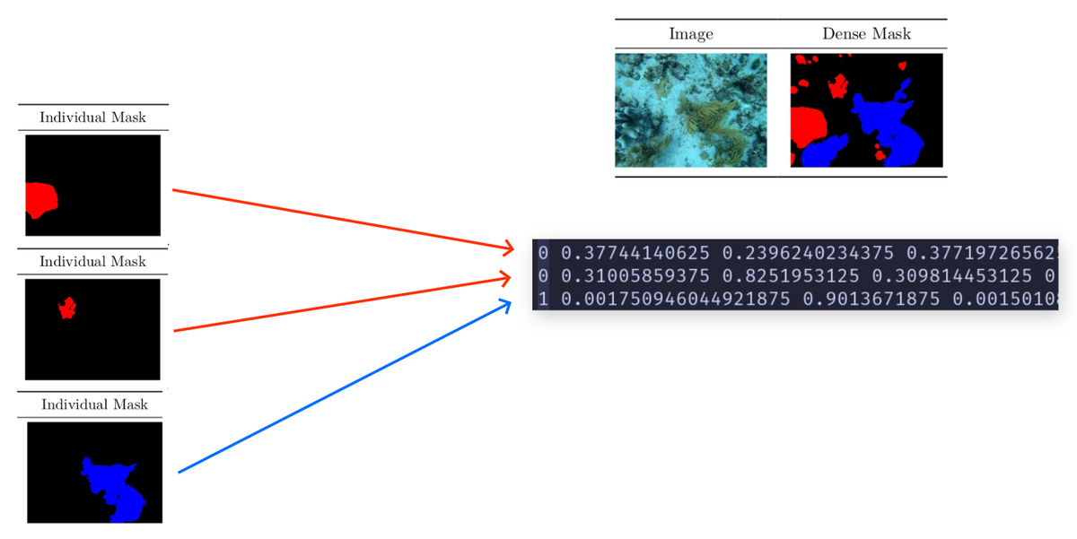 YOLOv8 TXT format conversion
Each line represents an instance of a class with a defined contour. It has the following format:
class_number x1 y1 x2 y2 x3 y3 ... xk yk
class_number x1 y1 x2 y2 x3 y3 ... xj yj
Where the coordinates x and y are normalized to the image width and height accordingly. Therefore, they always lie in the range [0,1].
Example:
1 0.617 0.359 0.114 0.173 0.322 0.654
0 0.094 0.386 0.156 0.236 0.875 0.134
Therefore, each line corresponds to an individual mask instance.
The OpenCV library is employed to convert the dense individual masks into contour coordinates.
Data Modeling
Data Split
In this section, we elucidate the methodology employed for the train/val/test splits across different datasets.
For each region, a dedicated dataset is created with an 80/10/10 split ratio
for train/val/test. Simultaneously, a comprehensive global dataset is
established using the same split ratios. Importantly, any image allocated to
the test set for a region-specific dataset is also included in the test set for
the global dataset (similarly for train and val splits). This design
facilitates the evaluation of models trained on region-specific datasets
against the global dataset.
| Dataset | Region | splits ratio | train | val | test | total |
|---|---|---|---|---|---|---|
| ALL | ALL | 80/10/10 | 1392 | 173 | 177 | 1742 |
| SEAFLOWER | BOLIVAR | 80/10/10 | 196 | 24 | 25 | 245 |
| SEAFLOWER | COURTOWN | 80/10/10 | 192 | 24 | 25 | 241 |
| SEAVIEW | ATL | 80/10/10 | 264 | 33 | 33 | 330 |
| SEAVIEW | IDN_PHL | 80/10/10 | 189 | 24 | 24 | 237 |
| SEAVIEW | PAC_AUS | 80/10/10 | 467 | 58 | 59 | 584 |
| TETES | PROVIDENCIA | 80/10/10 | 84 | 10 | 11 | 105 |
Instance Segmentation vs Semantic Segmentation
Semantic segmentation assigns a class label to each pixel in an image, such as ‘person,’ ‘dog,’ or ‘flower,’ grouping together pixels of the same class. Conversely, instance segmentation distinguishes between individual instances of objects within the same class, treating each one as a separate entity.
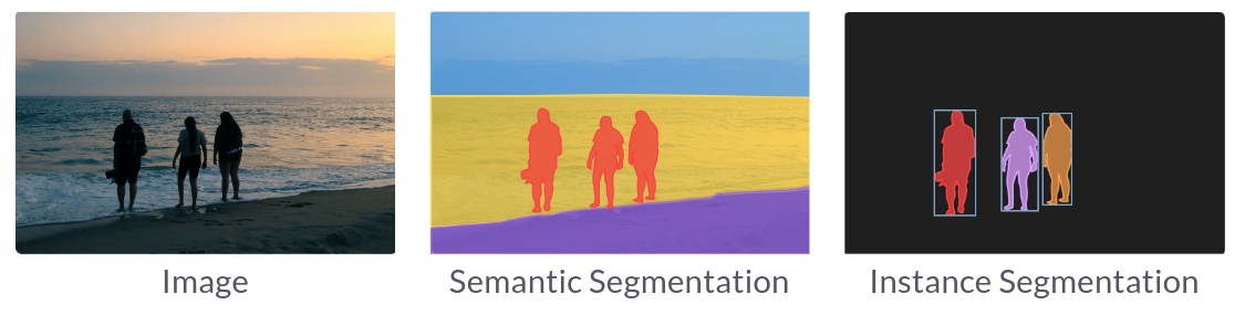 Semantic segmentation vs Instance segmentation
For analyzing benthic coral reefs, an instance segmentation approach proves superior as it enables precise localization and counting of reef organisms.
Evaluation Metrics
The mean Intersection Over Union (mIoU) and the Dice Coefficient were selected to evaluate the performance of the semantic segmentation results from the models. We stayed away from mean Precision Accuracy (mPA) as it can be very problematic in skewed datasets.
mIoU or Jaccard Index
In the context of semantic segmentation, the Jaccard Index is often referred to as the Intersection over Union (IoU) or the Jaccard similarity coefficient. It is a metric used to assess the accuracy of segmentation models by measuring the overlap between the predicted segmentation masks and the ground truth masks.
$$\mathit{IoU} = \dfrac{A \cap B}{A \cup B}$$The intersection is the number of pixels that are correctly predicted as part of the object, and the union is the total number of pixels predicted as part of the object by the model, including both true positives and false positives.
Higher Jaccard Index values imply better segmentation accuracy, indicating a greater overlap between the predicted and ground truth regions.
The Jaccard Index is commonly used as an evaluation metric for semantic segmentation models. Alongside metrics like pixel accuracy and class-wise accuracy, the Jaccard Index helps quantify the spatial agreement between the predicted and ground truth segmentation masks.
Dice Coefficient or F1 score
The Dice coefficient, also known as the Dice similarity coefficient or Dice score, is a metric commonly used in semantic segmentation to quantify the similarity between the predicted segmentation mask and the ground truth mask. It is particularly useful for evaluating the performance of segmentation models, especially when dealing with imbalanced datasets.
The Dice coefficient is calculated using the following formula:
$$\mathit{DiceCoefficient} = \dfrac{2 \times TP}{2 \times TP + FP + FN}$$Here’s how the terms are defined:
-
True Positives (TP): The number of pixels that are correctly predicted as part of the object by both the model and the ground truth. In segmentation, a true positive occurs when a pixel is correctly identified as belonging to the object.
-
False Positives (FP): The number of pixels that are predicted by the model as part of the object but are actually part of the background according to the ground truth.
-
False Negatives (FN): The number of pixels that are part of the object in the ground truth but are incorrectly predicted as background by the model.
The Dice coefficient essentially measures how well the model captures the true positives relative to the total pixels predicted as part of the object (both true positives and false positives) and the total pixels that actually belong to the object (true positives and false negatives). The factor of 2 in the numerator and denominator is used to ensure that the Dice coefficient ranges from 0 to 1.
A high Dice coefficient indicates a strong agreement between the predicted segmentation and the ground truth, while a low Dice coefficient suggests poor segmentation performance.
In summary, the Dice coefficient provides a way to balance and evaluate the trade-off between precision (capturing true positives) and recall (capturing all actual positives) in semantic segmentation tasks. It is a valuable metric, especially in cases of class imbalance where accuracy alone may not provide a clear picture of the model’s performance.
YOLOv8
Overview
We opted to utilize a pretrained YOLOv8 model and fine-tune it for our specific instance segmentation task. Renowned for its speed, accuracy, and user-friendly interface, YOLOv8 stands out as an ideal solution for various tasks, including object detection, tracking, instance segmentation, image classification, and pose estimation.
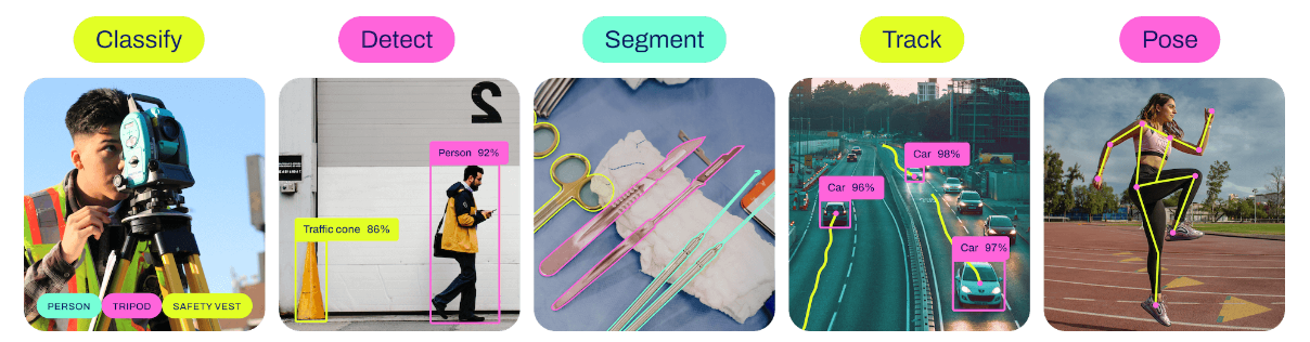 YOLOv8 Computer Vision Tasks
Training
Baseline
A baseline model was swiftly established to gauge the effectiveness of our approach and assess the potential performance enhancements that could be achieved. A medium size pretrained model is finetuned for 5 epochs on the train split.
| mIoU | IoU_hard | IoU_soft | IoU_other | mDice | Dice_hard | Dice_soft | Dice_other |
|---|---|---|---|---|---|---|---|
| 0.70 | 0.64 | 0.58 | 0.89 | 0.82 | 0.78 | 0.73 | 0.94 |
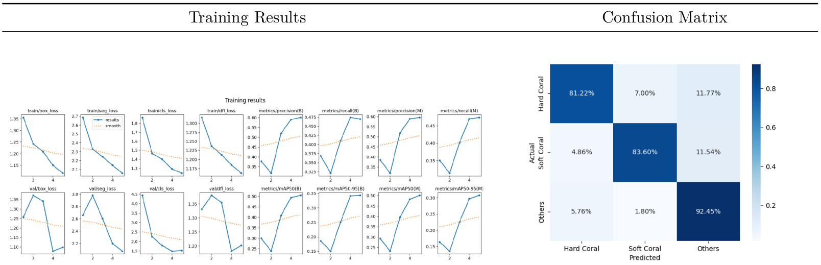 Results / Quantitative - Training metrics (left) and pixel level confusion matrix (right)
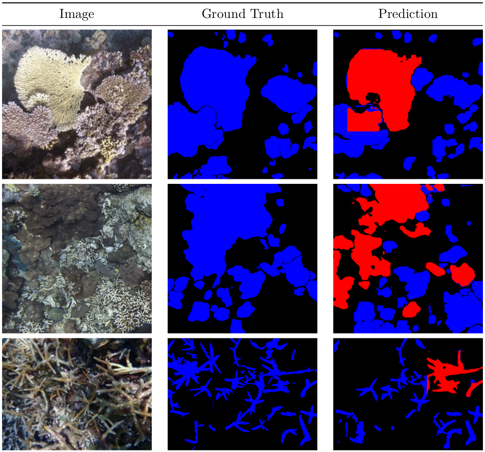 Results / Qualitative
The initial results are highly promising, prompting us to further optimize the performance of the modeling approach through meticulous selection of hyperparameters.
Best Model
In this section, we showcase the optimal models achieved through extensive fine-tuning efforts, involving hundreds of hours of GPU time to identify effective hyperparameter combinations.
Given the uncertainty about ReefSupport’s hardware configurations and the intended use of the models (including the possibility of running on live video streams from underwater cameras), we aimed to offer a diverse range of models. These span from models suitable for embedding on edge devices, enabling real-time video stream segmentation, to high-end GPUs delivering peak performance. This approach ensures flexibility to accommodate various deployment scenarios.
The pre-trained YOLOv8 models undergo fine-tuning for 140 epochs with images resized to 1024x1024 pixels. Additionally, random flipping and rotation of images up to 45 degrees are applied during training.
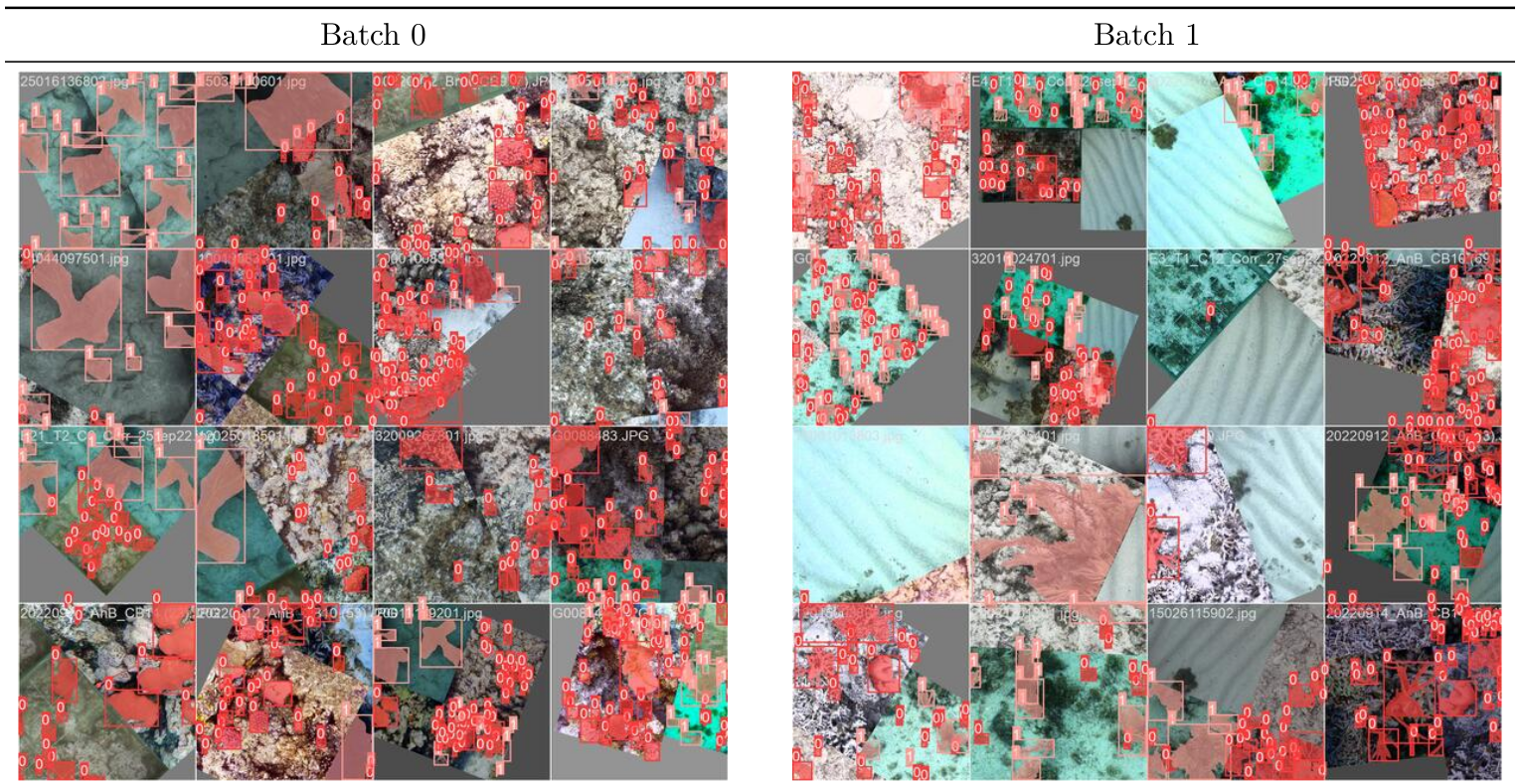 Data Augmentation / Batch Samples
| mIoU | IoU_hard | IoU_soft | IoU_other | mDice | Dice_hard | Dice_soft | Dice_other |
|---|---|---|---|---|---|---|---|
| 0.85 | 0.80 | 0.81 | 0.94 | 0.92 | 0.89 | 0.90 | 0.97 |
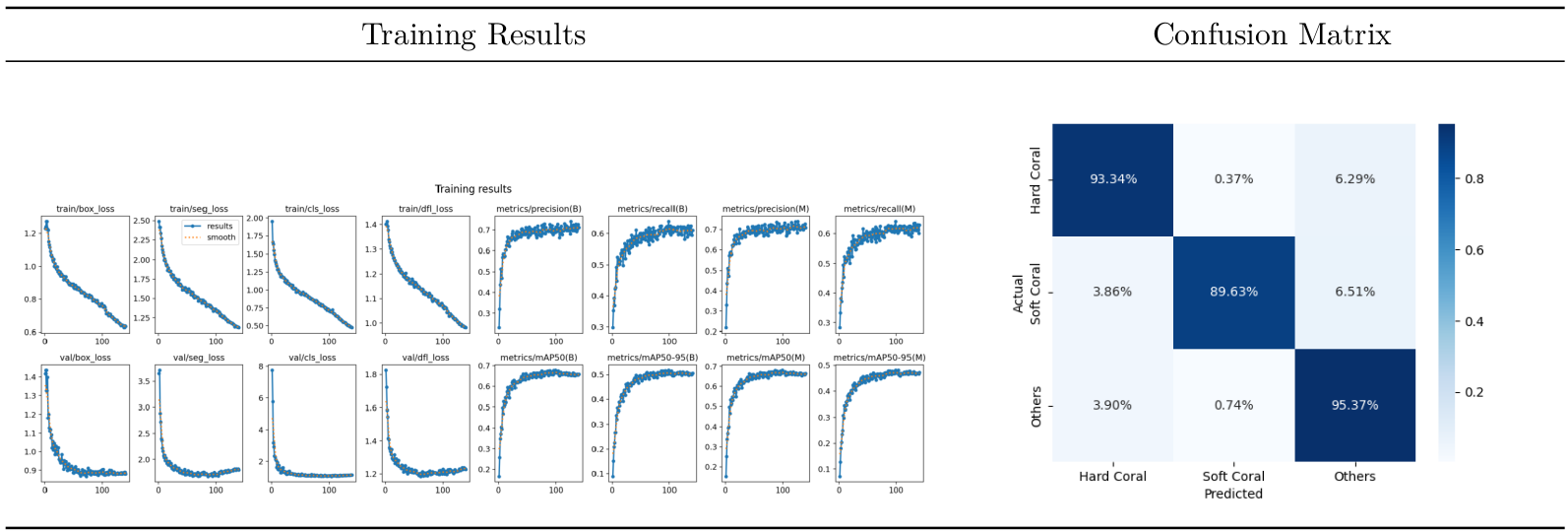 Results / Quantitative - Training metrics (left) and pixel level confusion matrix (right)
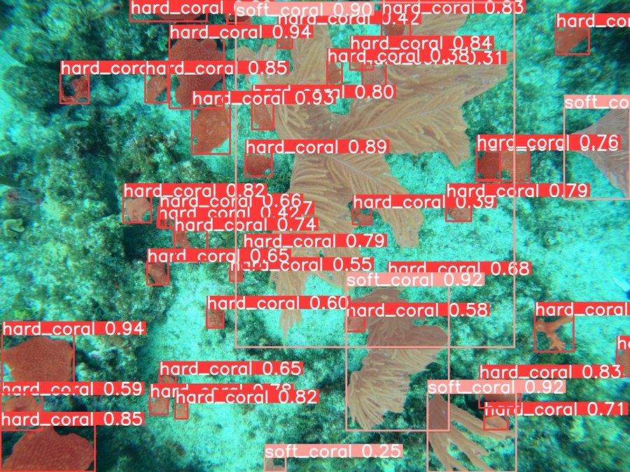
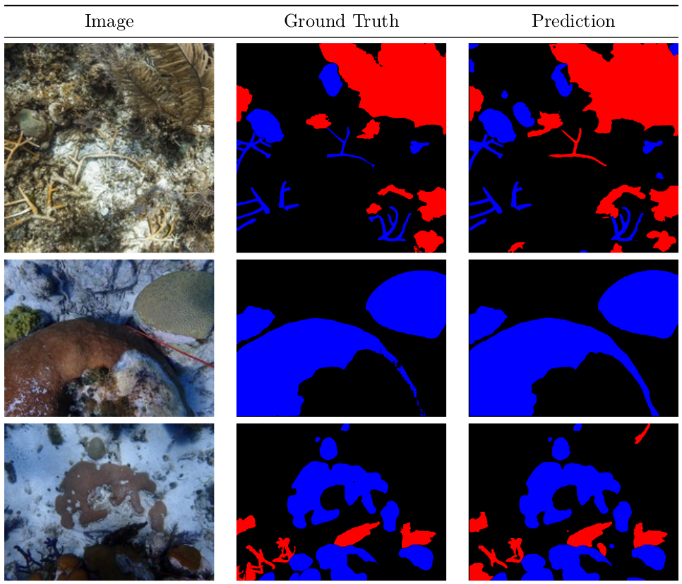 Results / Qualitative
Evaluation
The subsequent table provides a summary of the performance of the best model on the test sets for each region:
| data | mIoU | IoU_hard | IoU_soft | IoU_other | mDice | Dice_hard | Dice_soft | Dice_other |
|---|---|---|---|---|---|---|---|---|
| all | 0.85 | 0.80 | 0.81 | 0.94 | 0.92 | 0.89 | 0.90 | 0.97 |
| sf_bol | 0.80 | 0.85 | 0.63 | 0.93 | 0.89 | 0.92 | 0.77 | 0.97 |
| sf_crt | 0.72 | 0.70 | 0.54 | 0.94 | 0.83 | 0.82 | 0.70 | 0.97 |
| sv_atl | 0.78 | 0.63 | 0.78 | 0.92 | 0.87 | 0.78 | 0.87 | 0.96 |
| sv_phl | 0.62 | 0.75 | 0.21 | 0.91 | 0.72 | 0.86 | 0.34 | 0.95 |
| sv_aus | 0.69 | 0.76 | 0.38 | 0.92 | 0.79 | 0.86 | 0.55 | 0.96 |
| tt_pro | 0.87 | 0.77 | 0.88 | 0.96 | 0.93 | 0.87 | 0.94 | 0.98 |
As the various evaluation metrics are weighted in proportion to the number of pixels per region, we provide a summary below, illustrating the different weights assigned to regions based on their respective pixel counts:
| data | # images (test) | # pixels | weight (%) | mIoU | IoU_hard | IoU_soft | IoU_other |
|---|---|---|---|---|---|---|---|
| sf_bol | 25 | 7056000000 | 39.2 | 0.80 | 0.85 | 0.63 | 0.93 |
| sf_crt | 25 | 1912699566 | 10.6 | 0.72 | 0.70 | 0.54 | 0.94 |
| sv_atl | 33 | 1136559093 | 6.3 | 0.78 | 0.63 | 0.78 | 0.92 |
| sv_phl | 24 | 866520651 | 4.8 | 0.62 | 0.75 | 0.21 | 0.91 |
| sv_aus | 59 | 1944497328 | 10.8 | 0.69 | 0.76 | 0.38 | 0.92 |
| tt_pro | 11 | 5079158784 | 28.2 | 0.87 | 0.77 | 0.88 | 0.96 |
Model size vs Model accuracy
The table below summarizes the performance of the different YOLOv8 models that are trained on the same training set, using the same test set for evaluation.
| model size | mIoU | IoU_hard | IoU_soft | IoU_other | mDice | Dice_hard | Dice_soft | Dice_other |
|---|---|---|---|---|---|---|---|---|
| x | 0.85 | 0.79 | 0.81 | 0.94 | 0.92 | 0.88 | 0.90 | 0.97 |
| l | 0.85 | 0.80 | 0.81 | 0.94 | 0.92 | 0.89 | 0.90 | 0.97 |
| m | 0.85 | 0.80 | 0.80 | 0.94 | 0.92 | 0.89 | 0.89 | 0.97 |
| s | 0.84 | 0.78 | 0.80 | 0.93 | 0.91 | 0.88 | 0.89 | 0.98 |
| n | 0.83 | 0.77 | 0.80 | 0.93 | 0.91 | 0.87 | 0.89 | 0.97 |
The top-performing model is the l size model, as indicated in the table
above. As the model size decreases, there is a slight degradation in
performance—from a mIoU of 0.85 to 0.83. However, the advantage of smaller
models lies in their faster execution and compatibility with smaller hardware
devices.
Conclusion
In our investigation, YOLOv8 has emerged as an exceptionally suitable model for our dataset and the associated computer vision task, particularly in instance segmentation. Its remarkable performance, even on modest hardware configurations, positions it as an effective solution for resource-constrained environments. Moreover, YOLOv8 demonstrates real-time capabilities when applied to video streams, significantly enhancing its practical utility.
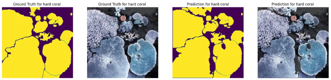 Benthic Segmentation / Hard Coral
In conclusion, while YOLOv8 presents a robust solution for the instance segmentation task, it is crucial to carefully address issues related to regional model performance, data leakage, and dataset quality. The insights gained from our findings are invaluable for refining and optimizing computer vision applications in marine biology and underwater image segmentation.
One can try out the model from the ML Space or directly from the snippet below: