On this page
Camera traps and field photos arrive by the thousand, and for conservation the first question is almost always the same: have we seen this animal before? Answering it — recognising an individual across time, cameras, and seasons — is called re-identification, and it underpins how researchers count populations, follow movements, and measure whether protection is working.
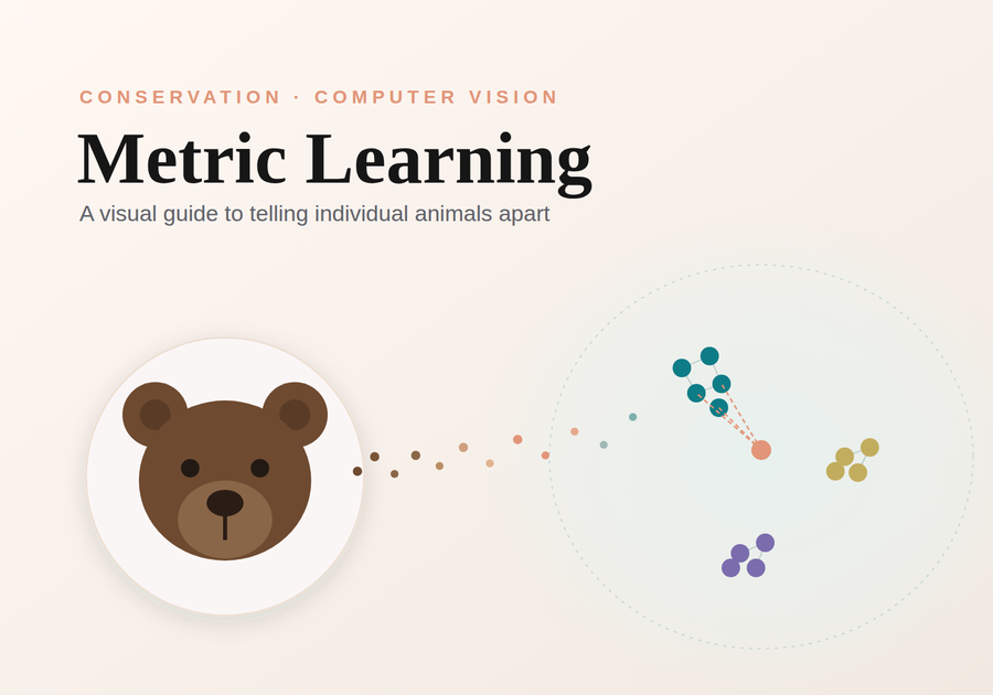
This is a visual, intuition-first tour of metric learning: the idea behind most modern re-identification systems. No heavy maths — just the shape of the problem and why this approach fits it so well.
The problem: a gallery that never stops growing
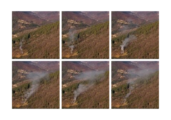
A wildlife population is not a fixed list. Cubs are born, individuals wander into a new valley, and a camera at Brooks Falls will happily photograph a bear no one has ever logged. The set of identities you care about is open and always growing — and at deployment you mostly meet individuals that were never in your training data.
The visual signal varies too. Brown bears carry no unique fur markings, so the clue lives in the face; trout and seals wear unique spot and coat patterns. Either way the task is identical: match this image to a known individual, or recognise that it is someone new.
Why classification hits a wall
The obvious first instinct is to train a classifier — one output per individual. That works for a small, fixed cast. But it breaks the moment the population grows: adding one individual means adding an output and retraining the whole model, and a classifier can never recognise someone it was never trained on. For an open, ever-growing set, that is a dead end.
 A classifier needs a slot per identity — a new individual means a retrain. Metric learning just drops another point into the space.
We need something that handles identities it has never seen before.
The core idea: turn images into points
Metric learning changes the question. Instead of predicting a label, we train a neural network to map each image to a vector — an embedding — and we shape that mapping so two images of the same individual land close together while different individuals land far apart.
So what is an embedding, concretely? Just a fixed-length list of numbers — a few hundred of them — that the network reads off each image.
 The embedding is simply a list of numbers (here 512 of them). That list is the coordinates of a single point in a 512-dimensional space.
Hundreds of dimensions sounds abstract, but the picture is the same as on a flat sheet of paper — just with more axes. Two points are “the same individual” when they sit close together.
 Each image becomes a point. Same individual, nearby points — identification turns into nearest-neighbour search.
That vector space is the embedding space, and once it exists, identification becomes geometry. Embed a new photo, then look at its nearest neighbours: if they are a known bear, it is probably the same bear; if everything nearby is far away, it is probably someone new. Adding an individual needs no retraining at all — you just store one more point. That is exactly why the approach scales to open populations.
How do we measure “close”? Two choices dominate — tap each:
Straight-line distance between two vectors. Intuitive, but sensitive to length — two embeddings can point the same way yet sit far apart if their magnitudes differ.
Measures the angle between two vectors, ignoring length. Two embeddings that point the same direction count as close regardless of magnitude — usually the better fit for normalized embeddings.
 Euclidean cares about length; cosine cares only about direction.
In practice embeddings are usually length-normalised, which makes cosine similarity the natural fit — only the direction of each vector carries the identity.
Shaping the space: a short history of losses
A network only learns this neat geometry if the training signal rewards it. That signal is the loss function, and the good ideas built on each other.
The original idea: take pairs. Pull two images of the same individual together; push two different individuals apart beyond a margin. Simple, but it judges each pair in isolation.
Look at three images at once — an anchor, a positive (same individual), and a negative (different one). Force the anchor closer to the positive than to the negative by a margin. Relative comparison beats absolute thresholds.
Not every pair deserves equal weight. Circle loss re-weights each similarity by how far it still has to move, giving a clearer, more adaptive decision boundary on noisy data.
Place every embedding on a sphere and add an angular margin between classes. Working with angles instead of raw distance carves crisp, well-separated regions — the go-to for faces.
 Pairs pull and push; triplets compare three at once; ArcFace separates identities by angle.
The story runs roughly like this. Contrastive loss starts with pairs — pull the same individual together, push different ones apart past a margin — but it judges each pair in isolation. Triplet loss adds context by comparing three images at once, asking only that the anchor sit closer to its positive than to its negative; relative comparisons turn out to be far more stable than absolute thresholds. Circle loss refines how hard each comparison is pushed, re-weighting by how far it still has to move. And ArcFace reframes everything in terms of angles on a sphere, carving crisp wedges between identities — which is why it has become the default for faces, including the bear face recogniser we will point to at the end.
Making it work in practice
A trained loss is only half the battle; the other half is which examples you show it.
 The hardest negatives — the ones that sneak inside the margin — carry the most learning signal.
Most pairs are easy — two obviously different animals tell the model nothing it does not already know. Hard negative mining deliberately seeks out the confusing cases: the lookalikes that slip inside the margin and produce the biggest learning signal. Strategies range from easy through semi-hard to fully hard, and choosing well makes training far more efficient on imbalanced field data.
Two more practical pieces complete the picture:
- Evaluation — accuracy@k / recall@k. Re-identification is a retrieval problem, so we ask a retrieval question: is the correct individual among the top k matches? Tracking accuracy@1, @5, and @10 reflects how the system is actually used — surface a short list of candidates for a human to confirm.
- Seeing the space. An embedding has far more than two dimensions, but it can be flattened into a 2-D picture so you can literally watch the clusters form as training proceeds — the quickest sanity check that the space is taking the shape you want.
 A projection tool like UMAP or t-SNE squeezes the 512 dimensions down to two while keeping near things near — turning an unviewable space into a map where the clusters jump out.
And the model itself is nothing exotic: a standard image-recognition network with a small extra layer added on to turn each picture into its embedding.
Where this shows up in conservation
This is the recipe behind our bear face recognition system — and the reason it generalises. The geometry never changes; only the data and the crop are species-specific. Swap brown bear faces for trout flanks or seal coats and the same machinery re-identifies a different animal.
It also sits alongside other identification approaches rather than replacing them. Where individuals carry rich local texture, matching keypoints directly with local feature matching is a strong alternative; metric learning instead learns a single global embedding per image. And whichever route you take, the result is only as good as the data feeding it — careful preparation of the crops and splits is what keeps the evaluation honest.
Try the interactive demo
See the model in action right in your browser — try it on the built-in examples or your own data. No install, no setup.
Open the demo