On this page
This blog post will detail the development process of an elephant rumble audio analyzer, created in partnership with The Elephant Listening Project.
Our vision is to conserve the tropical forests of Africa through acoustic monitoring, sound science, and education, focusing on forest elephants
– The Elephant Listening Project
For a comprehensive understanding of this project, one can read more on the detailed project page on passive acoustic monitoring for forest elephants.
What is sound?
🔉Sound is produced by variations in air pressure. These pressure variations can be measured and plotted over time to create a visual representation of the sound.
Sound waves often repeat at regular intervals, forming patterns where each wave has the same shape. The height of these waves, known as amplitude, indicates the intensity of the sound.
 A soundwave as a variation of air pressure
The time required for a signal to complete one full wave is called the period. The number of waves produced by the signal in one second is known as the frequency. Frequency is the reciprocal of the period and is measured in Hertz (Hz).
Most sounds we encounter do not follow simple, regular periodic patterns. However, signals of different frequencies can be combined to form composite signals with more complex repeating patterns. All the sounds we hear, including the human voice, are made up of such composite waveforms.
 Elephant rumble recorded in an african forest
Encoding sound digitally
To digitize a sound wave, the signal is converted into a series of numbers. This process involves measuring the amplitude of the sound at regular time intervals.
 Signal Sampling from Wikimedia
Each measurement is called a sample, and the sampling rate is the number of samples taken per second. For example, a common sampling rate is 44,100 samples per second. This means a 10-second music clip would contain 441,000 samples.
Human hearing range
👂The human ear can detect sounds within a specific range of frequencies, typically from about 20 Hz to 20,000 Hz (20 kHz). Sounds below this range are known as infrasounds, while sounds above this range are referred to as ultrasounds.
 Audible range for humans
Infrasounds, with frequencies below 20 Hz, are used by animals like elephants. Elephants communicate using these low-frequency sounds, which can travel long distances and penetrate through obstacles like dense vegetation.
On the other end of the spectrum, ultrasounds have frequencies above 20 kHz.
🦇 Bats are well-known for their use of ultrasound in echolocation. They emit high-frequency sound waves that bounce off objects and return as echoes, allowing bats to navigate and hunt in complete darkness.
Human hearing is limited compared to these examples, but our ability to perceive a wide range of frequencies is crucial for understanding speech, enjoying music, and detecting environmental sounds.
Spectrograms
A spectrogram is a visual representation of the frequency content of a sound signal over time. It provides a detailed picture of how the different frequencies present in the sound change and evolve.
To understand the relationship between a spectrogram and a raw audio waveform, let’s break down the process:
-
Raw Audio Waveform: The raw audio waveform is a plot of the amplitude of the sound signal over time. It shows how the pressure variations (which we perceive as sound) fluctuate. While the waveform gives a clear representation of the sound’s amplitude at each moment, it doesn’t provide detailed information about the frequency components of the sound.
-
Spectrogram: To create a spectrogram from the raw audio waveform, the sound signal is divided into small time segments, typically using a process called the Short-Time Fourier Transform (STFT). Each segment is analyzed to determine the frequencies present and their respective amplitudes.
 Fourier Transform Frequency View
In a spectrogram:
- The horizontal axis represents time.
- The vertical axis represents frequency.
- The intensity or color at each point represents the amplitude of a particular frequency at a given time.
This visualization allows us to see how the frequencies of a sound change over time. For example, in a speech signal, we can observe the varying frequencies produced by different phonemes, while in music, we can see the different notes and their harmonics.
Machine Learning and audio
State-of-the-art techniques in audio processing with machine learning convert raw waveforms into images and utilize computer vision methods. Most audio applications transform raw audio waveforms into spectrograms before inputting the data into vision models. Examples include the bird classifier BirdNet and Rainforest Connection, which help prevent illegal deforestation and perform bioacoustic monitoring.
As a result, spectrograms are vital in audio deep learning because they transform audio signals into a format that is more suitable for analysis by machine learning models, especially those based on deep learning techniques.
Here are several reasons why spectrograms are so important:
- Frequency-Time Representation: Spectrograms provide a detailed frequency-time representation of an audio signal, making it easier to analyze the frequency components and how they change over time. This is crucial for tasks such as speech recognition, music genre classification, and sound event detection, where understanding both the frequency content and temporal dynamics is essential.
- Visual Features: Many deep learning models, particularly convolutional neural networks (CNNs), are designed to work with visual data. Spectrograms convert audio data into a visual format, allowing these models to leverage their powerful feature extraction and pattern recognition capabilities. This visual representation helps the models learn complex patterns and structures in the audio signal.
- Noise Robustness: Spectrograms can help in distinguishing useful signal components from noise. By analyzing the frequency content, models can be trained to focus on relevant features and ignore irrelevant or noisy parts of the audio signal, improving the robustness and accuracy of the model.
- Task-Specific Adaptation: Different audio tasks may require focusing on different aspects of the audio signal. For example, speech recognition models might benefit from detailed time-frequency resolution, while music analysis might focus on harmonic content. Spectrograms can be adapted to highlight specific features relevant to the task, such as using Mel-spectrograms for speech and music applications.
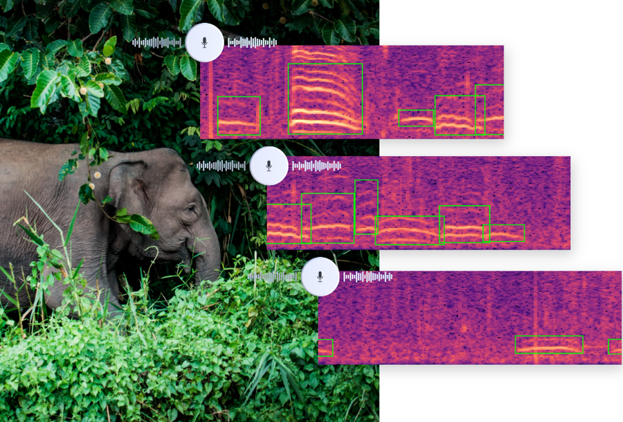
Elephant Rumbles
Elephant rumbles are low-frequency vocalizations produced by elephants, primarily for communication.
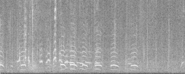
 Spectrogram of two elephant rumbles
- Two elephant rumbles are shown as stacks of parallel lines.
- The white line marks the upper boundary of infrasound, indicating frequencies below this line are inaudible to humans.
- The bracketed areas represent the speaking frequency ranges for men (70-200 Hz) and women (140-400 Hz).
- The stacks of lines above the white line represent the harmonics of the fundamental frequency, which in these calls is infrasonic.
Have a listen to the rumbles 🐘
These rumbles are a fundamental part of elephant social interactions and serve various purposes within their groups. Here’s a detailed explanation:
Characteristics of Elephant Rumbles
- Low Frequency: Elephant rumbles typically fall in the infrasound range, below 20 Hz, which is often below the threshold of human hearing. However, some rumbles can also be heard by humans as a low, throaty sound.
- Long Distance Communication: Due to their low frequency, rumbles can travel long distances, sometimes several kilometers, allowing elephants to communicate with each other across vast areas, even when they are out of sight. It can also travel through dense forests as the wavelength is very large.
- Vocal Production: Rumbles are produced by the larynx and can vary in frequency, duration, and modulation. Elephants use different types of rumbles to convey different messages.
Functions of Elephant Rumbles
- Coordination and Social Bonding: Elephants use rumbles to maintain contact with members of their herd, coordinate movements, and reinforce social bonds. For example, a matriarch might use a rumble to lead her group to a new location.
- Reproductive Communication: Male elephants, or bulls, use rumbles to communicate their reproductive status and readiness to mate. Females also use rumbles to signal their estrus status to potential mates.
- Alarm and Distress Calls: Rumbles can signal alarm or distress, warning other elephants of potential danger. These rumbles can mobilize the herd and prompt protective behavior.
- Mother-Calf Communication: Mothers and calves use rumbles to stay in contact, especially when they are separated. Calves may rumble to signal hunger or distress, prompting a response from their mothers.
Designing an ML pipeline to process large audio files
About 50 sound recorders are recording forest sounds around the clock in a forest in Congo. Terabytes of data are commonly generated in about a couple of months. Being able to process this amount of audio data fast and with accuracy is key to monitor the forest elephant population.
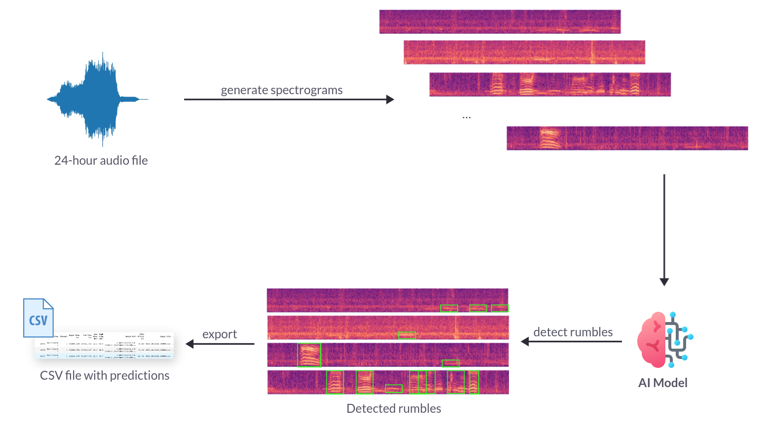 Overview of the ML pipeline to process audio files
The system must be capable of analyzing terabytes of data within a few hours. The primary bottlenecks in the data pipeline are:
- Spectrogram Generation: Converting raw audio into spectrograms that accurately capture the frequency range relevant for detecting elephant rumbles.
- Model Inference: Performing object detection on these spectrograms to identify elephant rumbles and report bounding boxes with associated probabilities.
To address these bottlenecks, the pipeline should:
- Generate spectrograms in the 0-250 Hz frequency range, which encompasses all elephant rumbles.
- Apply the rumble object detector to batches of these spectrograms.
- Save the detection results, including bounding boxes and probabilities, into a CSV file.
| Spectrogram | Prediction |
|---|---|
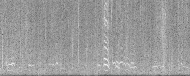
|
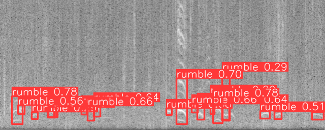
|
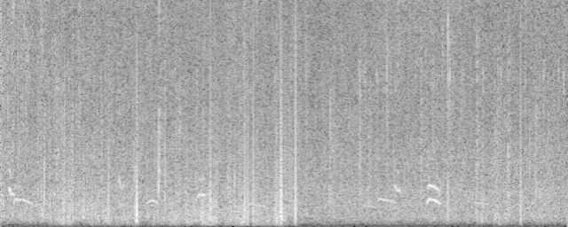
|
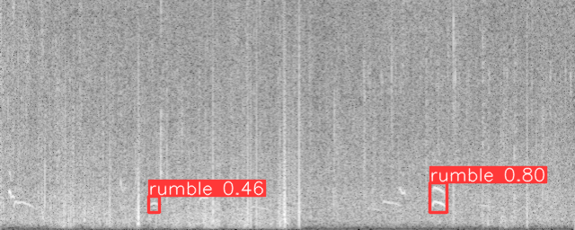
|
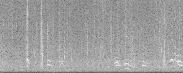
|
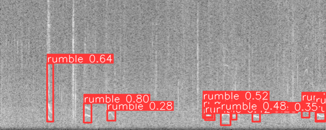
|
Below is a sample of a generated CSV file:
| freq_start | freq_end | t_start | t_end | probability | audio_filepath |
|---|---|---|---|---|---|
| 185.3 | 238.9 | 6.1 | 11.5 | 0.78 | data/08_artifacts/audio/rumbles/sample_0.wav |
| 187.4 | 237.1 | 107.4 | 112.3 | 0.77 | data/08_artifacts/audio/rumbles/sample_0.wav |
| 150.8 | 238.4 | 89.0 | 94.3 | 0.69 | data/08_artifacts/audio/rumbles/sample_0.wav |
| 203.1 | 231.6 | 44.1 | 47.5 | 0.65 | data/08_artifacts/audio/rumbles/sample_0.wav |
| … | … | … | … | … | … |
Provided dataset
The Elephant Listening Project provided hundreds of gigabytes of annotated audio files recorded in the African forest. These files were annotated using two distinct approaches. The first set was annotated using their current machine learning (ML) model, while the second set was meticulously annotated and reviewed by human experts. The annotations were exported from RavenPro, a comprehensive software tool for visualizing and analyzing audio recordings, widely used in bioacoustic research.
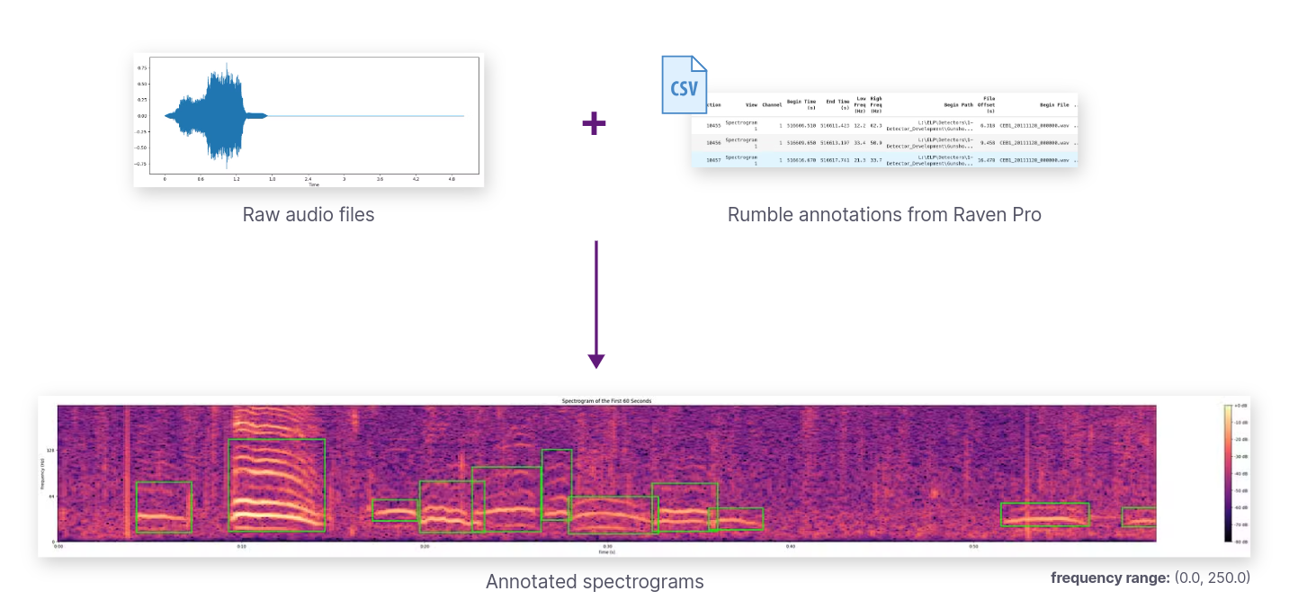 Provided dataset as raw audio files and annotations from RavenPro
The ML model-generated annotations typically identify most sound patterns within the 0-250 Hz frequency range but exhibit issues with overlapping rumbles and occasional false positives. Conversely, the human-curated dataset, though smaller, offers much higher quality annotations, despite some rumbles being unannotated. This meticulous attention to overlapping rumbles in the human annotations provides a valuable resource for training accurate ML models.
Given the higher quality of the human-curated dataset, we chose to use it for training and evaluating our ML models. To prepare the model inputs for training, the provided dataset needs to be transformed into an image dataset of spectrograms with bounding boxes that localize the rumbles.
Exploratory Data Analysis
Exploratory Data Analysis (EDA) is an approach to analyzing datasets to summarize their main characteristics, often employing visual methods. The primary goal of EDA is to uncover patterns, relationships, and anomalies in the data, which can then inform subsequent analysis or modeling tasks.
EDA typically involves the following steps:
- Data Collection: Gathering the relevant dataset(s) from various sources.
- Data Cleaning: Identifying and handling missing values, outliers, and inconsistencies in the data.
- Summary Statistics: Computing descriptive statistics such as mean, median, mode, standard deviation, etc., to understand the central tendencies and variability of the data.
- Data Visualization: Creating visual representations of the data using plots, charts, histograms, scatter plots, etc., to explore patterns, distributions, correlations, and trends within the data.
- Exploratory Modeling: Building simple models or using statistical techniques to further understand relationships within the data.
- Hypothesis Testing: Formulating and testing hypotheses about the data to validate assumptions or gain insights.
- Iterative Analysis: Iteratively exploring the data, refining analysis techniques, and generating new hypotheses as insights emerge.
EDA is a crucial initial step in any data analysis or modeling project as it helps analysts gain a deeper understanding of the dataset, identify potential challenges or biases, and inform subsequent analytical decisions. It provides a foundation for more advanced analyses, such as predictive modeling, hypothesis testing, or machine learning, by guiding feature selection, model building, and evaluation strategies.
Some key insights were derived from the exploratory data analysis:
- Rumble Duration: The typical duration of an elephant rumble ranges from 2 to 6 seconds, with some lasting up to 10 seconds. This information is crucial for determining the length and overlap of generated spectrograms.
- Frequency Range: All elephant rumbles occur within the 0-250 Hz frequency range. By focusing on this range, we can optimize spectrogram generation by excluding irrelevant frequencies.
- Communication Timing: Elephants primarily communicate with rumbles during dawn and dusk, when ambient noise is lower, allowing their low-frequency calls to travel more effectively. Consequently, the majority of our data points are concentrated at these times, which will guide our data splitting strategy.
Data split
We implemented a standard 80/10/10 data split on the provided dataset to ensure effective model evaluation. To prevent data leakage between training and testing phases, we meticulously split the audio files into non-overlapping time ranges. Each annotated audio file is divided into three distinct time segments: 80% of the rumbles are allocated to the training set, 10% to the validation set, and 10% to the testing set.
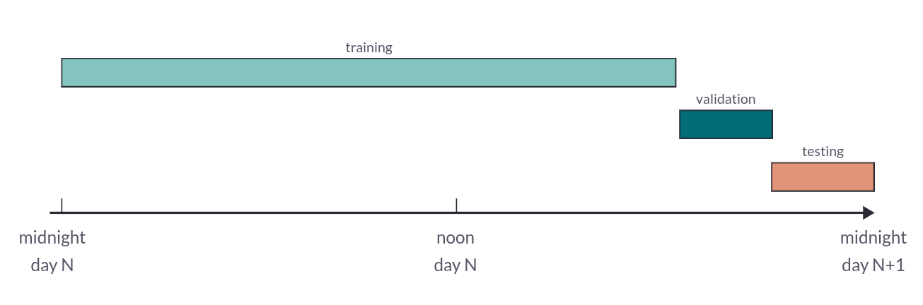 80/10/10 split of a 24 hour audio file in 3 non overlapping segments
Fast Spectrogram Generation
Spectrograms are a fundamental tool in audio analysis, providing a visual
representation of the spectrum of frequencies in a sound signal as it varies
with time. Generating spectrograms quickly and efficiently is crucial in
numerous applications such as speech recognition, music analysis, and
environmental sound classification. Fast spectrogram generation allows for
real-time processing and analysis of audio signals, which is essential in
scenarios where immediate feedback is necessary, such as live sound monitoring
and interactive audio applications.
Two powerful libraries for generating spectrograms in Python are librosa and
torchaudio.
Librosa
librosa is a widely-used library in the audio analysis
community, known for its user-friendly interface and comprehensive suite of
tools for audio processing. It provides robust functions for loading audio
files, computing spectrograms, and various other audio transformations.
![]() Librosa Logo
Librosa Logo
We began evaluating spectrogram generation using the librosa library. Loading raw audio files proved to be slow because librosa, by default, operates in a single-threaded manner, utilizing only one CPU core. Additionally, while generating spectrograms as images is time-consuming, the resulting visuals are highly aesthetic, thanks to the ability to apply various color maps.
 Spectrogram generated with Librosa
To enhance efficiency, we designed and implemented a multiprocessing pipeline that leverages all available CPU cores for loading audio files and generating spectrograms. On a 10-core machine, this approach resulted in approximately a tenfold increase in speed. However, maintaining such a multiprocessing pipeline can be complex. As an alternative, we considered using the torchaudio library, which natively supports multiprocessing and GPU acceleration. We aimed to compare the performance of both libraries to make an informed decision on the best approach for our needs.
TorchAudio
torchaudio, on the other hand, is a part of the PyTorch ecosystem, which
allows for seamless integration with deep learning models. It is optimized for
performance and can leverage GPU acceleration to speed up spectrogram
generation and other audio processing tasks.
![]() Torchaudio logo
Torchaudio logo
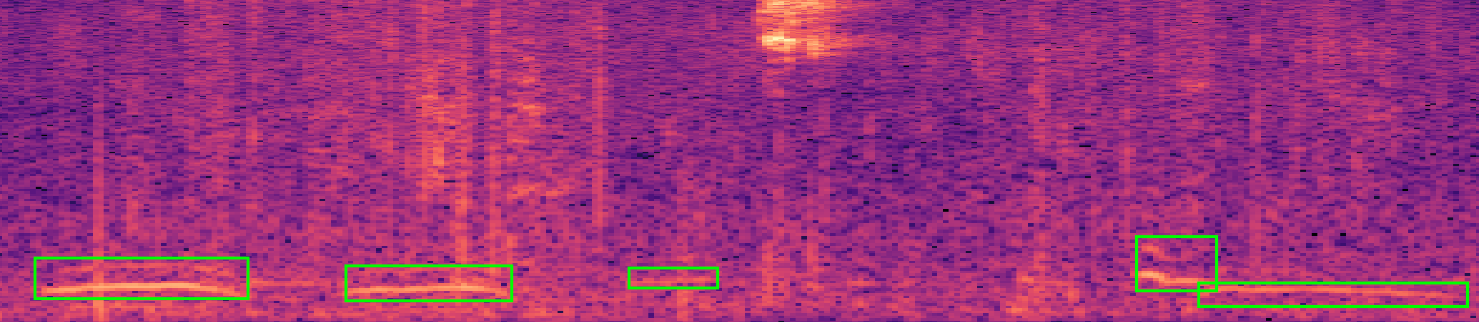
Loading raw audio files with torchaudio is significantly faster because it leverages multiple cores by default. Spectrogram generation is also much quicker than with librosa due to its optimized multiprocessing capabilities. Additionally, torchaudio can utilize GPU acceleration, further speeding up the process. After benchmarking both libraries, we decided to use torchaudio. This state-of-the-art audio processing library, which is part of the PyTorch ecosystem, offers robust performance and is well-maintained, making it the superior choice for our needs.
Loading a 24-hour raw audio file takes approximately 4 seconds, while generating 560 spectrograms to cover the entire recording takes around 11 seconds using torchaudio.
 Spectrogram generated with Torchaudio
Fast ML model inference
By adopting our approach, we have transitioned from dealing with raw audio data to addressing an object detection problem using spectrograms. Although there is a minor preprocessing cost involved in converting audio waveforms into spectrograms, this shift simplifies the problem to a well-understood computer vision challenge.

YOLO Overview
We opted to utilize a pretrained YOLOv8 model and fine-tune it for our specific object detection task. Renowned for its speed, accuracy, and user-friendly interface, YOLOv8 stands out as an ideal solution for various tasks, including object detection, tracking, instance segmentation, image classification, and pose estimation.
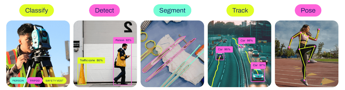 YOLOv8 Computer Vision Tasks
Spectrogram Generation and YOLOv8 Model Constraints
Pretrained YOLOv8 models require square images resized to 640 pixels. We face a trade-off between speed and accuracy when generating spectrograms. A smaller time range in each spectrogram yields higher resolution for detecting elephant rumbles, but requires generating more spectrograms to cover the entire time span.
Given that elephant rumbles typically last between 2 to 6 seconds, with some extending up to 10 seconds, a larger time range in a 640-pixel wide spectrogram can make these rumbles difficult to detect. To balance these factors, we decided to cover a 164-second time range in each 640-pixel wide spectrogram. Additionally, each spectrogram overlaps the next by 10 seconds, which corresponds to the maximum rumble duration and helps in deduplicating predicted rumbles.
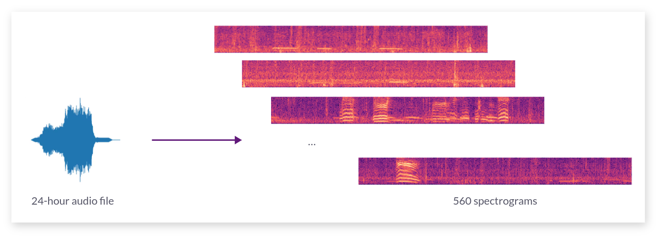 Generation of 560 spectrograms to cover the 24-hour time range
This approach results in the generation of approximately 560 spectrograms to cover a full 24-hour period.
Inference Speed and Performance Optimization
The model is designed to process batches of spectrograms simultaneously, utilizing multiprocessing when no GPU is available and leveraging GPU acceleration when present. Through experimentation, we determined an optimal batch size that balances memory usage with inference speed. With this setup, the model can process the 560 spectrograms in under 20 seconds on an 8-core machine and in under 4 seconds when using a GPU.
The table below provides a summary of the overall pipeline speed on a 24-hour audio file, highlighting the two key bottlenecks: spectrogram generation and model inference.
| Pipeline Step | GPU | CPU (8 cores) |
|---|---|---|
| Load the audio file | 4s | 4s |
| Generate the spectrograms | 11s | 11s |
| Run the model inference | 4s | 19s |
| Miscellaneous tasks | 1s | 1s |
| Total for a 24-hour audio file | 20s | 35s |
| Total for 1TB of audio data | 8.3h | 14.6h |
Analyzing months of audio recordings can now be done in a matter of hours, not weeks!
1 terabyte of audio data currently represents one month of recordings collected from 50 microphones distributed throughout the forest.
Conclusion 🐘
This article outlines the engineering approach used to develop a state-of-the-art elephant rumble detector with a strong emphasis on speed. Designing efficient data pipelines is crucial in conservation efforts, where vast amounts of data are continuously generated. The open-source tools developed in this project make a significant contribution to advancing global conservation initiatives. Moreover, the methods and techniques presented can be adapted to various conservation applications, including rare species identification and biodiversity monitoring.
One can try out the model from the live demo or directly from the snippet below: